Support and operation engineers don’t need to understand the majority of algorithms hidden in telecom software. But time to time it helps if you have an understanding of how some particular functionality is implemented.
The typical situation is Traffic Shaping or Overload Protection. Many operators want to understand and test, how their system behaves under a huge load of calls or messages. There are many ways how to implement these features, so let’s take a look at the most common ones.
Threshold
The easiest way how to protect the system is to define some limit. For example, we can say that our SBC is able to handle only 1.2 mil. parallel calls. If we receive a new invitate which exceeds this threshold, we respond with system error.
Similarly, we can set a limit for CPU or memory consumption. Whenever we reach, let’s say 60 % of the CPU we raise an alarm and don’t allow any new call/registration. As soon as the resource utilization drops below the threshold again, we can resume the standard system behavior and accept new calls.
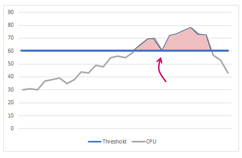
Sounds reasonable and simple, however, in case that the load is close to our limit – 60 % of CPU – it can lead to so called throttling causing system instability. The last thing which you desire for if you are facing high traffic.
Therefore, we can introduce two limits – Upper and Lower Watermarks.
Upper watermark is basically our threshold (60 % of CPU) which triggers rejecting of new calls. Lower watermark is a threshold below which the we have to fall (55 % CPU) in order to accept calls again.

If this is not good enough, we can also add a timeout defining the shortest time for which the system has to reject the calls even when we are under the lower watermark (e.g. 1 minute).
To achieve the smooth behavior of the system, we can have several of these overload thresholds (e.g. 3 – 60%, 75 %, 90 %) which are associated with progressively restrictive actions that help to maintain system resources and stability (e.g. no new registrations, no new calls, no call transfers, etc.).
Rate Limit
If we want to limit the amount of calls/messages per some interval, threshold itself is not sufficient. We can use Fixed or Sliding Window Counter. These algorithms are often used per particular subscribers (micro-policers) or interfaces.
Fixed Window Counter splits time in intervals. In each interval we allow only Limit number of messages. If the Limit is spent at the beginning of the interval, the new messages are dropped. However, if messages are sent at the end of the interval and the load continues in the next time slot, we can process more messages than is the Limit. That may lead to bursts of traffic.


Fixed-lenght window alghoritm
Sliding Window Counter makes sure, that we have never processed more than Limit number of messages in any given interval.


Floating window alghoritm
That improves the message distribution (hence stability of the system), but as we need to store timestamps of messages, this approach is not suitable for higher loads.
(Single) Token Bucket
Traffic shaping of lots of data is a task for Token Bucket Algorithm. You can find its description on wikipedia and many other webs. Its main advantage is that is not too complex and can used for aggregated (huge) traffic. Note, that particular implementation may use different terminology. Moreover, one thing is to understand the basic idea, the other to understand the constraints given by the actual implementation.
In Token Bucket algorithm we are using a couple of terms and definitions:
- Rate, Rate Limit
- Defines average throughput for the system, e.g. how many calls/messages per second system can process.
- Rate says how many Tokens are added into the Bucket in each interval.
- Burst, Burst Size
- Determines maximum number of messages that can be accepted by system in one step of the algorithm.
- Bucket, Bucket Size
- Contains Tokens which are spent for messages/calls. If there is no token left in Bucket, we have to drop new messages.
- If the traffic is low and we still have a space in the Bucket, we can store the unused Tokens.
- Meaning may differ implementation to implementation. Usually Bucket Size = Burst Size, but you can also find systems where Bucket Size = Rate Limit or Bucket Size = Rate Limit + Burst Size. It is essential to understand, what is the true meaning of Bucket Size in your system, as it gives the maximum number of messages that can be processed in one step.
- Token
- A virtual currency that we spend for messages. One token equals one message.
- Message
- Any type of packet or data frame. Can be used for any protocol (bits per sec, arp, ssh, udp, sip, ..). If we want to limit the number of calls, we typically limit the number of initial SIP INVITE messages.
The basic idea is very simple. The system can deliver X messages per second. Therefore, every second we add X tokens in the Bucket. If we receive more messages than is the actual number of tokens in the Bucket, the messages are dropped. If we receive less, we can store unused tokens in the Bucket. But not above the size of the Bucket.
Burst Size says, how many messages can be delivered above the limit (how many tokens above the limit we can store). In overload situation we receive every second less tokens than messages. This extra credit (Burst Size – Rate Limit) is quickly spent and we have to wait until the traffic drops again, so that we can store some spare tokens.
So let’s have an example:
Rate Limit = 12 msgs/s
Burst Size = 18 msgs/s
Therefore Bucket Size = 18
Every second we start with the actual number of tokens in the Bucket, plus we add another 12 tokens (Start Bucket). Then we receive some messages to process. As long as be we enough tokens in the bucket we can deliver them. Once all tokens are spent, messages are dropped.

The observation we can make, is that we can always deliver at least Rate Limit number of messages. On the other hand we can never deliver more than Burst Size. Also, if there is any burst of traffic, we can go over the Rate Limit only for a short period of time.

The issue with this description is, that in real life, 1 second is too much for our systems. We typically add Rate Limit/1000 number of tokens every millisecond (or equally we add a new token every 1/Rate Limit second). That means, we count with uniform distribution of messages. Which, as you may feel, is not always the case.
That’s why it can happen that even when our limit is 12 msgs/s, we process less messages, if all of them are sent at the beginning of 1 second interval (similar to Fixed Window Counter). That’s also one of the reasons why we need to define the Burst Size – that is the size of our Buffer, which can help to overcome short bursts (and drops) of traffic.
In real systems the values could look like this:
Rate Limit = 1 250 000 msgs/s; hence we add 1 250 tokens every 1 ms
Burst Size = 1 500 msgs
We can’t process more than 1 500 msgs per 1 ms. If an overload occurs, the average maximum rate of processed messages should be close to 1 250 000 msgs per second.

Burst Size value generally depends on available resources and variation of traffic. The easist way how to derive a reasonable initial Bucket Size is based on three-sigma rule of thumb. Of course, depending on your traffic profile, the limit can be adjusted later.
To sum up, the Single Token Bucket algorithm is a perfect solution, if you need to support Service Level Agreements (SLAs) defining guaranteed average rate. That can be extremely useful in a multi – tenancy environment, but can be applied in any kind of traffic shaping scenario. There are also many variants of this algorithm, which can deal with various priorities of traffic data or longer bursts of traffic.
